Overview

This project maps CO₂ emissions across Europe. The aim is to estimate an emissions inventory for each of the ~116 000 administrative jurisdictions across Europe and the UK.

The model spatially disaggregates each country's official (Eurostat) CO₂ emissions inventory to places using OpenStreetMap. Vehicle emissions are attributed across fuel stations, train emissions at stations, aviation bunker fuel emissions at airports, and so on. Industrial source emissions are located at the registered address where these emissions phyiscally occur or are legally controlled. Data are for the year 2018.

Downloads

The dataset is available in tabular, raster and vector formats. The data are for the year 2018. Emissions are reported in units of metric tonnes (t) CO₂.

The version provided at this page is OpenGHGMap R2021A.

Interactive map

An interactive visualization of the latest version of the dataset is available at: https://openghgmap.net

Summary results

Emissions estimates for cities and states are available in Excel format and text format. The summary file contains results for each administrative level, and the 'onlycities' files contain results for just the most detailed admin level in each country. (The latter file is intended to help with municipal-level analyses, since municipalities may be defined at various levels, typically around 7-10, in different countries.) Region population estimates are taken from GHS-POP.

Excel file with all admin levels: allcountries_summary.xlsx
Excel file with only the highest detail admin level (just cities): allcountries_onlycities_summary.xlsx
TSV file: allcountries_summary.zip (tab-delimited; UTF-8 encoded)

This download provides the total emisions in each region, itemized using the following categories:

1. Airports
2. Buildings (emissions from building heating and light commercial activity)
3. Industrial facilties (ETS)
4. Farms
5. Vehicles (fuel stations)
6. Harbours
7. Refineries
8. TiOx production
9. Train stations

Gridded raster format

A gridded version of the dataset is available as a GeoTIFF in EPSG:4326 equirectagular / plate carrée projection.

This data product will be published later in the year.

Shapefile vector format

This zip file provides GeoJSON files with results per administrative unit. The GeoJSON features provide the spatial extent (polygon) and properties for each region including the name, total CO₂ emissions of the region (in tonnes), emisisons itemized by category, and a list of ETS-registered facilities. These regions are taken from OpenStreetMap. At the present time we do not offer results in the NUTS system.

Note: Each feature is a single polygon. Regions which consist of multiple polygons will occur multiple times; that is, regions do not use FeatureCollections or MultiPolygons.

Note: The visualization presented at this website has been adjusted to account for the fact that administrative levels are not used in the same way across countries. The web visualizaton shows different levels in different countries to promote usability. For example, in most countries level 8 corresponds to municipalities, but in the UK level 8 is not used so level 10 is displayed instead.

Download: allcountries.geojson.zip (924 MB)

Validation and Comparison

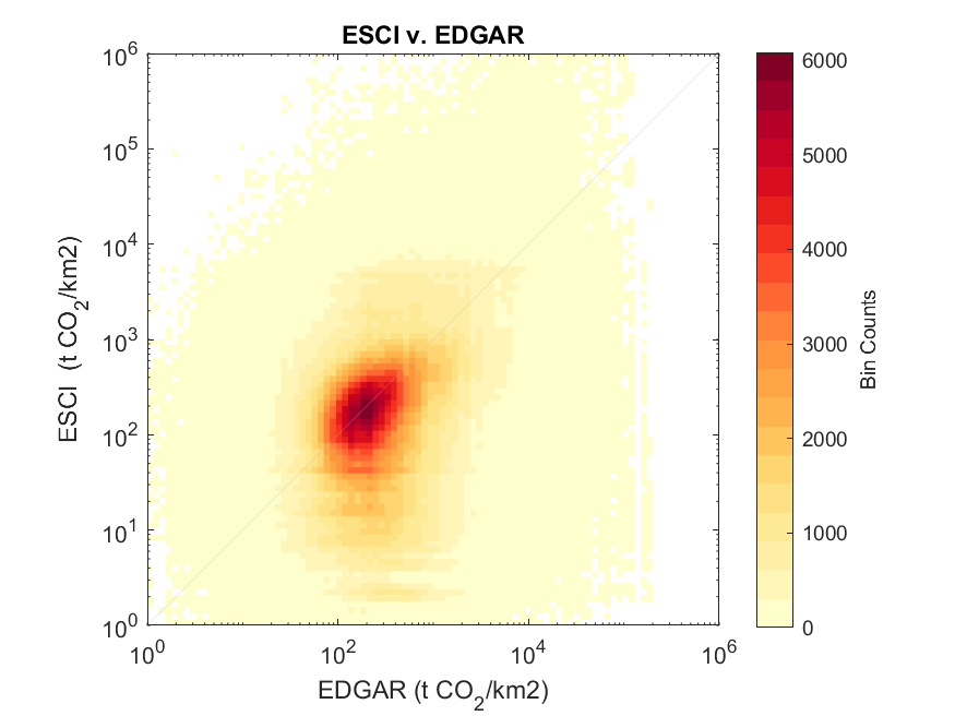
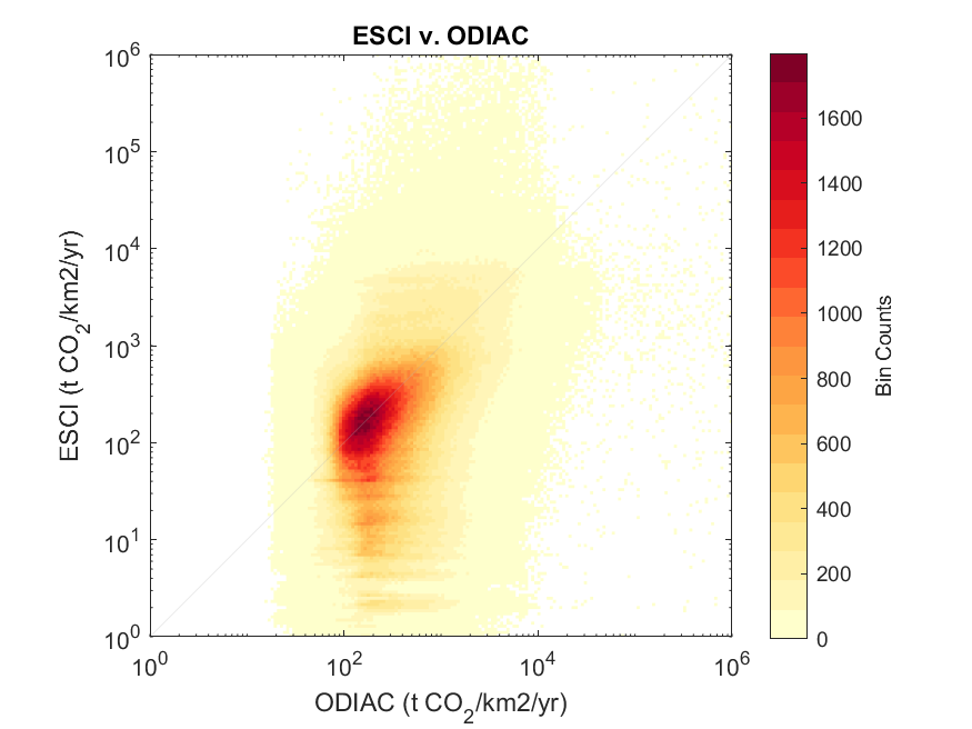
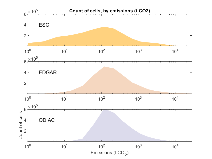
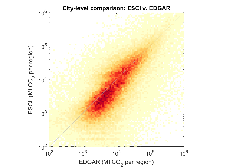
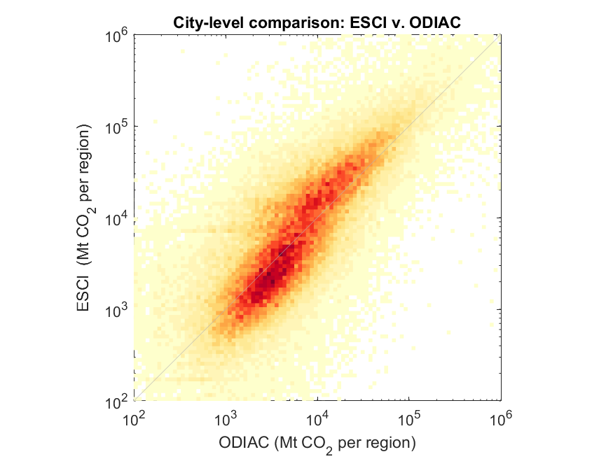
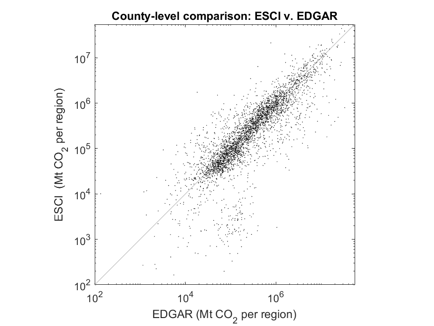
Two other prominent spatial GHG inventories covering Europe are the JRC EDGAR and ODIAC models. A thorough intercomparison has not yet been conducted. However to provide an initial validation it is useful to compare the results of the three models. The comparison indicates that the results are broadly comparable across the three models, but OGM reveals higher variability emissions per grid cell compared to the other two models.

Why use this model? In addition to introducing a new approach for mapping emissions based on OpenStreetMap, OpenGHGMap provides results per administrative jurisdiction.

Comparison at the grid cell level

Comparison at the city level

Comparison at the county level (one administrative level above cities)

This table provides an overview of the OGM model together with EDGAR, ODIAC, and the Global Carbon Project's GridFED model.

	Resolution	Temporal resolution	Itemization	Results by jurisdiction	Scope	Method synoposis
OpenGHGMap	Point-source, 1km grid, and per municipality	Annual	167 CRF categories, using, 9 spatialization methods	Country, State, County, Municipality, facility	Europe	Spatialize national emissions using activity data from OpenStreetMap
ODIAC	1km	Monthly	Total emissions	Country	Global	Spatialize national emissions using nighttime lights and power plant locations
EDGAR v6.0	0.1° (11km×11km cells at the equator)	Hourly	31 IPCC CRF categories	Country	Global	Collected activity-level data sources (e.g steel industry, FAO for farming activity, ship and flight tracks)
GCP-GridFED	0.1° (11km at the equator)	Monthly	Total emissions, per 5 fossil fuels	Country	Global	Use JRC EDGAR map to spatialize GCP's national inventory

Methodology

The methodology is presented in this open-access publication:

Moran, D., Pichler, P.-P., Zheng, H., Muri, H., Klenner, J., Kramel, D., Többen, J., Weisz, H., Wiedmann, T., Wyckmans, A., Strømman, A. H., and Gurney, K. R.: Estimating CO2 Emissions for 108,000 European Cities, Earth Syst. Sci. Data 14, 845-864. 2022. https://doi.org/10.5194/essd-14-845-2022
The methods for each emissions categories can be summarized as follows:

• Industrial facilities Facilities with large point source emisisons must obtain permits and provide an address to the EU Emissions Trading System. This registered address is typically for the facility itself or a nearby office, but in some cases it may be an address for a headquarters (e.g. emissions at Norwegian offshore platforms are registered to corporate offices in Stavanger).
• Vehicles Total national emissions from all vehicles (personal & commercial) are allocated evenly across fuel stations in the country.
• Buildings These emissions from residential and commercial buildings, light manufacturing, and households primarily arise from fossil fuel heating and from fossil fuel combustion activites which are not large enough to require registration with the EU ETS (e.g. operating boilers, heaters, generators, etc.). These are allocated evenly across all buildings registered in OpenStreetMap (these appear as grey dots when zoomed in to cities). This category ecompasses the following CRF codes:
  • 1.A.2.G - Fuel combustion in other manufacturing industries and construction
  • 1.A.4.A - Fuel combustion in commercial and institutional sector
  • 1.A.4.B - Fuel combustion by households
  • 1.D.3 - Biomass - CO₂ emissions (memo item)
  • 2.D.3 - Other non-energy product use
• Airports Emissions from on-airport operations (vehicles, building heating, etc) plus emissions from aircraft bunker fuel are allocated to airports across each country weighted by the volume of total passenger traffic handled at that airport. Bunker fuel use by military aviation is included, but will be located at conventional airports as no data on military air traffic (estimated by some to be 15% of all air traffic) is available. (Note that a more refined aviation emissions model is presently under development at NTNU.)
• Farms This model focuses on CO₂ emissions from fossil fuels and excludes emissions from biomass burning (including wood-fired stoves) and biological exchange processes such as soil emissions. These emissions correspond to the following three CRF categories: Fuel combustion in agriculture, forestry and fishing (1.A.4.C), liming (3.G), and urea application (3.H). These emissions are allocated evenly across all polygons in the national EU CORINE land-use map which are marked as farm.
• Harbours Emissions from marine bunker fuel and in-harbour operations are allocated evenly across harbours. It is planned to upgrade this module in the near future to use a spatial shipping emisisons model under development at NTNU. These emissions correspond to the two CRF categories "fuel combustion in domestic navigation" (1.A.3.D) and "international navigation" (memo item 1.D.1.B).
• Trains Total emissions from trains are allocated evenly across all stations in the country.
• Refineries This category contains any residual discrepancy between the sum of ETS-registered emissions and the corresponding total industrial emissions reported to Eurostat.

Overview of Coverage

This table provides an overview of the coverage of countries and administrative levels. The administrative levels used in OpenStretMap are documented here but generally level 1 refers to countries, levels 2 and 3 are unused, levels 4 and 5 correspond to states (NUTS-2), levels 6-7 cover counties, and levels 8 and up cover municipalities and sub-municipality divisions such as neighborhoods or parishes. Note that in the interactive map visualization the level displayed has been adjusted in some cases to promote ease of use.

	Administrative level
Country	4	5	6	7	8	9	10
Austria	9	-	94	-	2107	-	-
Belgium	3	-	14	43	581	-	-
Bulgaria	28	-	-	270	-	-	-
Croatia	-	-	21	530	-	-	-
Cyprus	-	-	5	-	65	-	-
Czech republic	8	-	14	77	6778	-	-
Denmark	5	-	-	100	-	-	-
Estonia	-	-	15	79	-	4097	-
Finland	19	-	19	70	312	-	-
France	13	-	97	320	34882	-	-
Germany	16	30	401	1215	11013	-	-
Great britain	3	9	155	-	-	-	11522
Greece	8	14	75	330	-	-	-
Hungary	3	7	20	176	3156	-	-
Iceland	-	8	68	-	-	15	-
Ireland and northern ireland	-	3	26	-	103	-	-
Italy	20	-	104	111	7920	-	-
Latvia	4	-	119	-	-	-	-
Liechtenstein	-	-	2	-	11	-	-
Lithuania	10	60	517	-	-	-	-
Luxembourg	-	-	12	-	105	-	-
Malta	5	-	-	-	67	-	-
Netherlands	12	-	-	-	358	-	-
Norway	13	-	-	356	-	-	-
Poland	17	-	380	2478	-	-	-
Portugal	7	39	18	307	-	-	-
Romania	42	-	-	6	664	-	-
Slovakia	8	-	-	-	79	-	-
Slovenia	-	-	-	14	210	-	-
Spain	19	-	48	-	8156	-	-
Sweden	22	-	-	294	-	-	-
Switzerland	26	10	142	38	2214	-	-
Turkey	81	-	974	-	-	-	-
Ukraine	27	-	258	274	5007	-	-

Contributors and Funding Acknowledgements

The team behind this project consists of: Daniel Moran¹ (PI), Peter-Paul Pichler², Helene Muri¹, Jan Klenner¹, Diogo Kramel¹, Heran Zheng¹, Anders Hammer Strømman¹, Annemie Wyckmans¹, Johannes Többen², Helga Weisz², Thomas Wiedman³ Kevin R. Gurney⁴,

¹ Norwegian University of Science and Technology (NTNU)
² Potsdam Institute for Cimate Impact Research (PIK)
³ University of New South Wales
⁴ Northern Arizona University

We gratefully acknowledge funding from the Research Council of Norway under grant #287690.

This resource is built using data from OpenStreetMap, © OpenStreetMap contributors, and in parts utilizing shapefiles from Eurostat © EuroGeographics for the administrative boundaries

This model is open data. It is licensed under the Open Data Commons Open Database License (ODbL). You are free to re-use this data for any purpose, but any derived data must use the same, or similar, license as the ODbL. For more on the license please read the OSM's page about copyright and license.